A Parallel Maze Generation Algorithm
The Hilbert Lookahead Algorithm
The discovery
I stumbled across this interesting algorithm going by the name “Hilbert Lookahead Algorithm” in this video on generating mazes in Minecraft.
I found this particularly intriguing, since I would not have imagined it possible to generate mazes in an embarrasingly parallel way, under the constraints that the maze should:
- Not have any isolated regions—i.e. any node should be reachable from any other node.
- There should be no cycles.
These constraints, on the surface, seem to require at least some form of global coordination, however as demonstrated in the video, that is not the case.
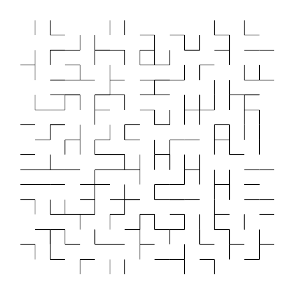
For example, if we use the most naïve parallel maze generation algorithm possible:
N = 16
grid = np.array(list(product(range(N), repeat=2)))
fig, ax = plt.subplots(1, 1, figsize=(6,6))
np.random.seed(0)

for i in range(len(grid)):
    dir = np.random.randint(0, 4)
    match dir:
        case 0:
            dir = (0, 1)
        case 1:
            dir = (1, 0)
        case 2:
            dir = (0, -1)
        case 3:
            dir = (-1, 0)
    ax.arrow(*grid[i], *dir, head_width=0, head_length=0)

ax.axis("off")
ax.set_aspect(1)
plt.tight_layout()
plt.savefig("invalid_maze.png", transparent=True)
We will almost guaranteed get an invalid maze, and a very bad one at that:
The idea
If we have a predefined space-filling curve, we can use this to generate a valid maze using the following insight:
If all nodes only select a single edge to that connects to a node with a higher order in the space-filling curve, there cannot exist cycles, and all edges must meet at the final node in the space-filling curve.
If we at the same time maintain that nodes can only connect to their 4-neighbors (up/down/left/right), then we get a square grid, connected by edges such that there are no isolated regions (disjoint subgraphs) or cycles. That is a valid maze!
Probably the most famous space-filling curve is the “Hilbert Curve”:
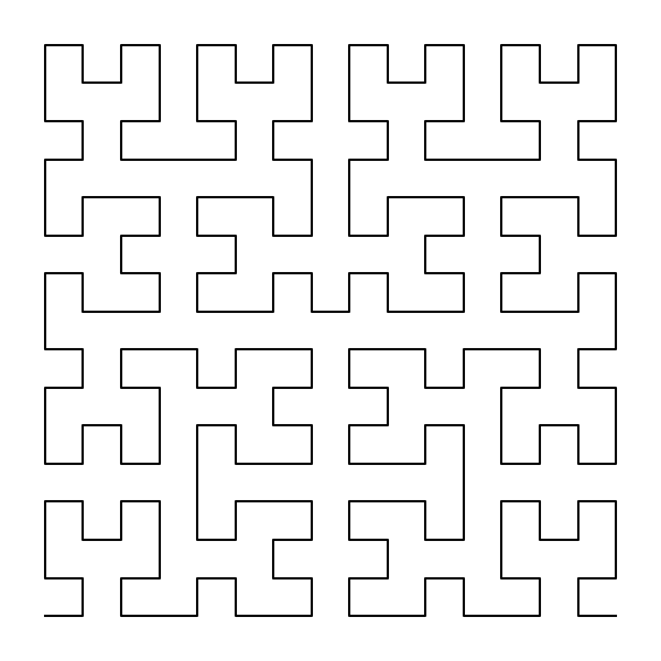
Of particular note here, is that the Hilbert Curve is deterministic for a given size, meaning that in principle any information about the Hilbert Curve can be accessed in parallel.
The Hilbert Curve
Luckily for us, there exists an easy way to generate the Hilbert Curve (here implemented by ChatGPT because I am lazy):
def rot(s, x, y, rx, ry):
    """
    Rotate/flip a quadrant as part of the Hilbert index algorithm.
    """
    if ry == 0:
        if rx == 1:
            x = s - 1 - x
            y = s - 1 - y
        return y, x
    return x, y

def xy2d(N, x, y):
    """
    Convert (x, y) in [0..N-1] x [0..N-1] to a Hilbert index d in [0..N^2-1].
    N must be a power of 2.
    """
    d = 0
    s = N // 2
    while s:
        rx = 1 if (x & s) else 0
        ry = 1 if (y & s) else 0
        d += s * s * ((3 * rx) ^ ry)
        x, y = rot(s, x, y, rx, ry)
        s //= 2
    return d
If we look at the second function xy2d, we see that it calculates the order of a single coordinate—perfect for parallelization, further establishing the choice of the Hilbert Curve.
As an aside, here is how I created the Hilbert Curve in the figure above:
N = 16
grid = np.array(list(product(range(N), repeat=2)))
order = np.array([xy2d(N, x, y) for x, y in grid]).argsort()
hilbert_curve = grid[order]

plt.figure(figsize=(6, 6))
plt.plot(*hilbert_curve.T)
plt.gca().axis("off")
plt.gca().set_aspect(1)
plt.tight_layout()
plt.savefig("hilbert_curve.png", transparent=True)
The algorithm
Now that we have established the ground-work, we can sketch out the algorithm. Instead of writing the algorithm out, as it should be completely local, in order to be embarrassingly parallel, I will simply write the rule we use:
Assume we have access to a function calculating the Hilbert Index of any coordinateH(x,y)(xy2d)
- Given a node (vertex) with coordinates (
x,y), calculate it's Hilbert IndexH' = H(x,y).- For each neighbor in the 4-neighborhood of the original node with coordinates, (
x + dx,y + dy), check ifH' < H(x + dx, y + dy), and select a random neighbor that satisfies.
That is all. So simple 🎉.
Implementation
As with the algorithm itself, the implementation is exceedingly simple. For simplicity, I’ll abstract it into three functions:
def four_neighbors(N, x, y):
    """
    Return the valid four-neighbors of a node in a NxN grid.
    """
    return [
        (nx, ny)
        for dx, dy in [(1, 0), (-1, 0), (0, 1), (0, -1)]
        if 0 <= (nx := x + dx) < N and 0 <= (ny := y + dy) < N
    ]

def hilbert_lookahead_local_rule(N, x, y):
    """
    The local rule for the Hilbert Lookahead Algorithm.
    """
    return [
        (nx, ny)
        for nx, ny in four_neighbors(N, x, y)
        if xy2d(N, x, y) <= xy2d(N, nx, ny)
    ]

def hilbert_lookahead_maze(N, seed=None):
    """
    For each vertex, compute its Hilbert index.
    Then, for every vertex, create a directed edge to exactly one neighbor
    (up, down, left, right) whose Hilbert index is larger (chosen at random).
    """
    random.seed(seed)
    return {
        (x, y) : random.choice(hilbert_lookahead_local_rule(N, x, y))
        for x, y in product(range(N), repeat=2)
        if (x, y) != (N - 1, 0) # Last vertex has node edges
    }
However, as you can see the local rule of the Hilbert Lookahead Algorithm can be applied locally, meaning that the algorithm is indeed embarrassingly parallel!
Let’s try to use it:
Success 🎉🎉
Further investigation
I wanted to look a bit deeper into how this algorithm works, and which algorithms it can produce, and I also had an idea for an animation of the algorithm—but let’s take one thing at a time.
The possibility space
If we look at all the edges that fulfill the two rules of the Hilbert Lookahead Algorithm, we might be able to spot some patterns. Again finding these edges is trivial:
def valid_hilbert_lookahead_choices(N):
    """
    For each cell, list all neighbors that have a larger Hilbert index.
    Returns a list of directed edges ( (x,y), (nx,ny) ).
    """
    valid_edges = []
    for x, y in product(range(N), repeat=2):
        for nx, ny in hilbert_lookahead_local_rule(N, x, y):
            valid_edges.append(((x, y), (nx, ny)))
    return valid_edges
Which we quickly visualize:
N = 16
fig, (ax1, ax2) = plt.subplots(1, 2, figsize=(12,6))

all_edges = valid_hilbert_lookahead_choices(N)

for (x, y), (nx, ny) in all_edges:
    dx, dy = nx - x, ny - y
    ax1.arrow(x, y, dx, dy, head_width=0, head_length=0)
However, this visualization is not super helpful, other than saying that all edges in the grid can technically be selected. In reality, not all edges are equally likely. Since we select a single valid edge from each node, and nodes have between (0)1-3 edges originating from them, edges from nodes with 1 edge in total are guaranteed to be selected, while edges from nodes with 2 edges in total are more likely to be selected than those from nodes with 3 edges in total:
edge_counts = {}
for xy, _ in all_edges:
    if xy not in edge_counts:
        edge_counts[xy] = 1
    else:
        edge_counts[xy] += 1

for (x, y), (nx, ny) in all_edges:
    dx, dy = nx - x, ny - y
    match (dx, dy):
        case (0, 1):
            dcol = "red"
        case (1, 0):
            dcol = "green"
        case (0, -1):
            dcol = "blue"
        case (-1, 0):
            dcol = "orange"
        case _:
            raise RuntimeError("Unknown direction")
    ax2.arrow(
        x, y, dx * 0.75, dy * 0.75,
        head_width=0.15, head_length=0.15,
        color=dcol if edge_counts[(x,y)] != 1 else "black",
        alpha=(4-edge_counts[(x,y)])/3,
        linewidth=(4-edge_counts[(x,y)])/2
    )

ax1.axis("off")
ax1.set_aspect(1)
ax2.axis("off")
ax2.set_aspect(1)
plt.tight_layout()
plt.savefig("hilbert_lookahead_possibilities.png", transparent=True)
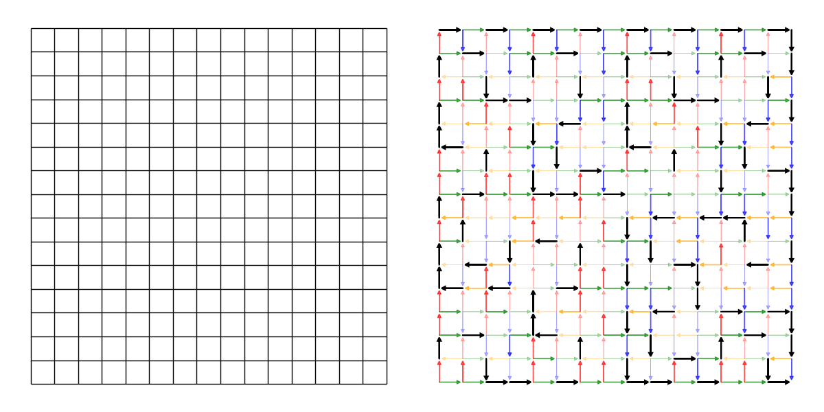
As can be seen, there are many edges which are always selected, many which are selected 50% of the time and many which are selected 33% of the time.
Maze quality
When I saw the the pattern above I immediately questioned whether the generated mazes are any good. So to test it, I quickly asked ChatGPT (again laziness) to give me a search algorithm, to find the solution and it came up with this:
def build_undirected_adjacency(edges):
    """
    Convert directed edges {u: v} into an undirected adjacency list.
    """
    adj = defaultdict(list)
    for u, v in edges.items():
        adj[u].append(v)
        adj[v].append(u)
    return adj

def bfs_path(adj, start, goal):
    """
    Find a path from start to goal in the undirected graph using BFS.
    """
    queue = deque([(start, [start])])
    visited = set([start])
    while queue:
        node, path = queue.popleft()
        if node == goal:
            return path
        for nxt in adj[node]:
            if nxt not in visited:
                visited.add(nxt)
                queue.append((nxt, path + [nxt]))
    return None
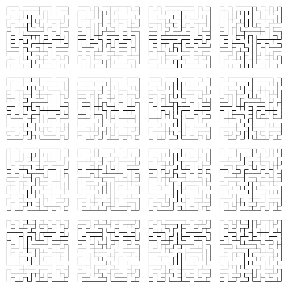
Which looks good enough for this purpose. Let’s try it out on the 16 mazes generated earlier:
N = 16

fig, axs = plt.subplots(4, 4, figsize=(12, 12))

for i, ax in enumerate(axs.flatten()):
    edges = hilbert_lookahead_maze(N, seed=i)
    adj = build_undirected_adjacency(edges)
    path = bfs_path(adj, (0, 0), (N - 1, N - 1))
    for (x, y), (nx, ny) in edges.items():
        ax.arrow(x, y, nx - x, ny - y, head_width=0, head_length=0)
    for (x, y), (nx, ny) in zip(path, path[1:]):
        end = (nx, ny) == (N - 1, N - 1)
        ax.arrow(
            x, y,
            nx - x, ny - y,
            head_width=0.125 if end else 0,
            head_length=0.125 if end else 0,
            linewidth=2,
            color="red"
        )
    ax.axis("off")
    ax.set_aspect(1)

plt.tight_layout()
plt.savefig("4x4_solution.png", transparent=True)
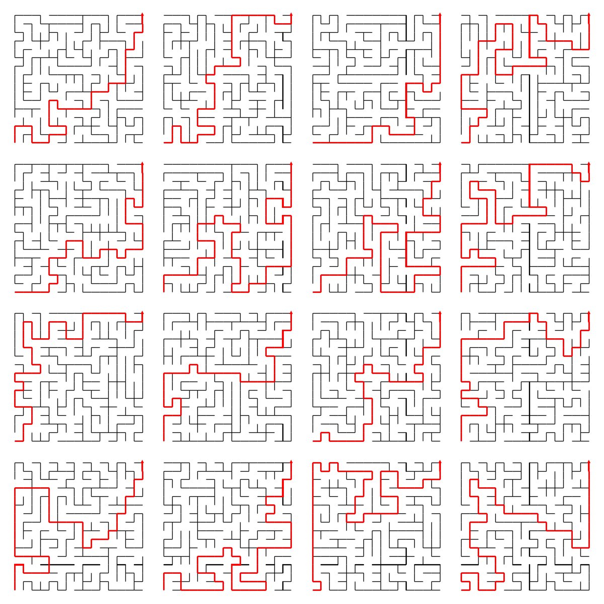
That actually looks pretty good to me.
Putting it all together
From the moment I saw the original video that showcased the Hilbert Lookahead Algorithm, I wanted to create a nice visualization of the algorithm in action, as it seemed like a fun challenge and the visualization I had in my head looked great (at least from my minds eye 😉).
The visualization pulls together all the elements from this post in a single snappy—if I have to say so myself—animation:
And here comes the (pretty long) matplotlib code for creating the animation—great learning experience though:
## Animation helpers
def uv_lerp(start, end, t):
    (x0, y0), (x1, y1) = start, end
    rad_start, rad_end = math.atan2(y0, x0), math.atan2(y1, x1)

    # Shortest path from rad_start to rad_end (mod 2 * pi)
    diff = rad_end - rad_start
    if diff > math.pi:
        diff -= 2 * math.pi
    elif diff < -math.pi:
        diff += 2 * math.pi
    # Interpolate angle
    rad_cur = rad_start + diff * t

    return math.cos(rad_cur), math.sin(rad_cur)

def ease_in_out(t: float) -> float:
    return 0.5 * (1 - math.cos(math.pi * t))

# Animation main function
def animate(
        N=8,
        seed=42,
        epoch_frames=10,
        epoch_pause=3,
        easing=ease_in_out
    ):
    """
    Animated transition between the four steps:
      1) All possible valid edges
      2) Highlighted chosen edges
      3) Static full maze structure
      4) Animated BFS solution path
    """
    if isinstance(epoch_frames, int):
        epoch_frames = [epoch_frames] * 3
    if isinstance(epoch_pause, int):
        epoch_pause = [epoch_pause] * 3

    fig, ax = plt.subplots(figsize=(N // 2, N // 2))

    ax.set_xticks([])
    ax.set_yticks([])
    ax.set_xlim(-1, N)
    ax.set_ylim(-1, N)
    ax.set_aspect('equal')
    ax.axis('off')

    # Step 1: Compute all possible valid edges
    curve = hilbert_curve(N)
    valid_edges = valid_hilbert_lookahead_choices(N)
    edges = hilbert_lookahead_maze(N, seed)
    adj = build_undirected_adjacency(edges)
    path = bfs_path(adj, (0, 0), (N - 1, N - 1))

    # Prepare drawing elements
    hilbert_edges : dict[
            tuple[int, int],
            tuple[mpatches.FancyArrow, float, float, float, float]
        ] = dict()
    for (x1, y1), (x2, y2) in zip(curve, curve[1:]):
        arrow = ax.arrow(
            x1, y1, x2 - x1, y2 - y1,
            color='black', linewidth=0.5, alpha=0.8,
            head_width=0, head_length=0,
            animated=True
        )
        hilbert_edges[(x1, y1)] = (arrow, x1, y1, x2 - x1, y2 - y1)


    edge_arrows : list[
            tuple[mpatches.FancyArrow, float, float, float, float]
        ] = []
    # Draw all valid edges in color depending on their direction
    for (x1, y1), (x2, y2) in valid_edges:
        dx, dy = x2 - x1, y2 - y1
        match (dx, dy):
            case (0, 1):
                dcol = "red"
            case (1, 0):
                dcol = "green"
            case (0, -1):
                dcol = "blue"
            case (-1, 0):
                dcol = "orange"
            case _:
                raise RuntimeError("Unknown direction")
        arrow = ax.arrow(
            [], [], [], [],
            color=dcol, linewidth=0.75, alpha=0.6,
            head_width=0.125, head_length=0.125,
            animated=True
        )
        edge_arrows.append((arrow, x1, y1, dx * 0.75, dy * 0.75))

    chosen_edges : dict[
            tuple[int, int],
            tuple[mpatches.FancyArrow, float, float, float, float]
        ] = dict()
    for (x1, y1), (x2, y2) in edges.items():
        arrow = ax.arrow(
            [], [], [], [],
            color='black', linewidth=1.5, alpha=0.8,
            head_width=0, head_length=0,
            animated=True
        )
        chosen_edges[(x1, y1)] = (arrow, x1, y1, x2 - x1, y2 - y1)

    bfs_path_lines : list[
            tuple[mpatches.FancyArrow, float, float, float, float]
        ] = []
    if path:
        for i in range(len(path) - 1):
            x1, y1 = path[i]
            x2, y2 = path[i + 1]
            dx, dy = x2 - x1, y2 - y1
            arrow = ax.arrow(
                [], [], [], [],
                color='red', linewidth=3,
                head_width=0, head_length=0,
                animated=True
            )
            bfs_path_lines.append((arrow, x1, y1, dx, dy))

    # Update function helper functions and globals
    def draw_elems(elems):
        list(map(lambda x : ax.draw_artist(x[0]), elems))

    def remove_elems(elems):
        list(map(lambda x : x[0].remove(), elems))

    # Precompute end of each animation step
    fends = [5]
    for i in range(3+3):
        if i % 2 == 0:
            fends.append(fends[-1] + epoch_frames[i // 2])
        else:
            fends.append(fends[-1] + epoch_pause[i // 2])
    edge_added = set()
    arrow_removed = set()

    # Animation function
    def update(frame):
        # List for storing elements scheduled for
        # deletion/addition in current frame
        add_elems = []
        del_elems = []

        # Draw Hilbert Curve before initializing animation
        if frame < fends[0]:
            if frame == 0:
                add_elems += list(hilbert_edges.values())
        # Step 1: Draw all valid edges
        elif frame < fends[1]:
            epoch_end, epoch_start = fends[1], fends[1] - epoch_frames[0]
            epoch_len = epoch_end - epoch_start - 1
            epoch_i = frame - epoch_start
            epoch_f = epoch_i/epoch_len

            # Expand each arrow from the vertices
            for arrow, x, y, dx, dy in edge_arrows:
                arrow.set_data(
                    x=x,
                    y=y,
                    dx=dx * easing(epoch_f),
                    dy=dy * easing(epoch_f)
                )
            # Add all arrows at start of step (epoch)
            if epoch_i == 0:
                add_elems += edge_arrows
        elif frame < fends[2]:
            # Fade out Hilbert Curve in-between steps
            epoch_end, epoch_start = fends[2], fends[2] - epoch_pause[0]
            epoch_len = epoch_end - epoch_start - 1
            epoch_i = frame - epoch_start
            epoch_f = epoch_i/epoch_len
            for arrow, _, _ , _ , _ in hilbert_edges.values():
                arrow.set_alpha(1 - epoch_f)
                if epoch_f == 1:
                    del_elems.append((arrow, ))
            pass
        # Step 2: Collapse to single instantiation of maze
        elif frame < fends[3]:
            epoch_end, epoch_start = fends[3], fends[3] - epoch_frames[1]
            epoch_len = epoch_end - epoch_start - 1
            epoch_i = frame - epoch_start
            epoch_f = epoch_i / epoch_len
            # Fade the selected edges in
            for arrow, x, y, dx, dy in chosen_edges.values():
                dist = ((2 * x/(N - 1) - 1)**2 + (2 * y/(N - 1) - 1)**2)**(1/2)
                dist_f = min(1, max(0, 3 * epoch_f - 2**(1/2) * dist))
                # Add the edges when they fade in
                if dist_f > 0:
                    if (x, y) not in edge_added:
                        edge_added.add((x,y))
                        add_elems.append((arrow, ))
                    arrow.set_data(
                        x=x,
                        y=y,
                        dx=dx*dist_f,
                        dy=dy*dist_f
                    )
                    arrow.set_alpha(dist_f)
            # Rotate the possible edges onto the selected edge and fade out
            for arrow, x, y, dx, dy in edge_arrows:
                _, _, _, sdx, sdy = chosen_edges[(x, y)]
                dist = ((2 * x/(N - 1) - 1)**2 + (2 * y/(N - 1) - 1)**2)**(1/2)
                dist_f = min(1, max(0, 3 * epoch_f - 2**(1/2) * dist))
                dx_adj, dy_adj = uv_lerp((dx, dy), (sdx, sdy), easing(dist_f))
                dx_adj *= 0.75
                dy_adj *= 0.75
                if dist_f > 0 and (x, y) not in arrow_removed:
                    # Remove the arrows when they fade out
                    if dist_f == 1:
                        arrow_removed.add((x, y))
                        del_elems.append((arrow, ))
                    arrow.set_alpha(0.6 * (1 - dist_f ** 4))
                    arrow.set_linewidth(0.75 * (1 - dist_f ** 4))
                    arrow.set_data(
                        dx=dx_adj,
                        dy=dy_adj,
                        head_width=0.125*(1 - dist_f),
                        head_length=0.125*(1 - dist_f)
                    )
        elif frame < fends[4]:
            pass # Pause
        # Step 4: Draw BFS solution path
        elif frame < fends[5]:
            epoch_end, epoch_start = fends[5], fends[5] - epoch_frames[2]
            epoch_len = epoch_end - epoch_start
            epoch_i = frame - epoch_start + 1
            epoch_f = epoch_i / epoch_len
            last_epoch_f = (epoch_i - 1) / epoch_len

            # Extract the solution segment to be added in the current frame
            bfs_so_far = bfs_path_lines[
                max(0, math.floor(len(bfs_path_lines) * last_epoch_f) - 1)
                :
                math.ceil(len(bfs_path_lines) * epoch_f)
            ]
            # For each edge in the current solution segment
            for bi, (arrow, x, y, dx, dy) in enumerate(bfs_so_far):
                # Check if it is the leading edge in the solution
                is_last = bi == (len(bfs_so_far) - 1)
                # Calculate length of the leading edge
                if is_last:
                    length = (len(bfs_path_lines) * epoch_f) % 1
                    if length == 0:
                        length = 1
                else:
                    length = 1
                # Display the solution (as an arrow if leading)
                arrow.set_data(
                    x=x,
                    y=y,
                    dx=dx*length,
                    dy=dy*length,
                    head_width=0.125 if is_last else 0,
                    head_length=0.125 if is_last else 0
                )
                add_elems.append((arrow, ))
                ## Remove edge(s) under solution from:
                ## (x, y) -> (x+dx, y+dy) or (x + dx, y + dy) -> (x, y)
                # Case 1
                if (x, y) in chosen_edges:
                    forward = chosen_edges[(x, y)]
                    forward_arrow : mpatches.FancyArrow = forward[0]
                    if forward[3:5] == (dx, dy):
                        forward_arrow.set_data(
                            x=x+dx,
                            y=y+dy,
                            dx=-dx*(1-length),
                            dy=-dy*(1-length)
                        )
                        if length == 1:
                            forward_arrow.set_linewidth(0)
                            forward_arrow.set_color("white")
                # Case 2
                if (x+dx, y+dy) in chosen_edges:
                    backward = chosen_edges[(x+dx, y+dy)]
                    backward_arrow : mpatches.FancyArrow = backward[0]
                    if backward[3:5] == (-dx, -dy):
                        backward_arrow.set_data(
                            x=x+dx,
                            y=y+dy,
                            dx=-dx*(1-length),
                            dy=-dy*(1-length)
                        )
                        if length == 1:
                            backward_arrow.set_linewidth(0)
                            backward_arrow.set_color("white")

        # Remove/Add scheduled elements
        remove_elems(del_elems)
        draw_elems(add_elems)
        return []

    # Create the animation
    total_frames = fends[-1]
    anim = animation.FuncAnimation(
        fig, update,
        frames=TQDM(range(total_frames), desc="Rendering..."),
        interval=50, blit=True
    )

    # Formatting
    ax.xaxis.set_visible(False)
    ax.yaxis.set_visible(False)
    ax.set_frame_on(False)
    fig.patch.set_alpha(0.)
    plt.tight_layout(pad = 0.05)

    # If running in a script, you might want:
    writer = animation.HTMLWriter(
        metadata=dict(artist='Asger Svenning'),
        fps=15,
        bitrate=200
    )
    anim.save(
        'animated_transition.htm',
        writer=writer,
        savefig_kwargs={"transparent": True, 'facecolor': 'none'},
        dpi=100
    )
    plt.close()
animate(N=32, seed=123, epoch_frames=[15, 75, 75], epoch_pause=7)
I should also warn that it was quite annoying trying to embed the .htm animation in Jekyll, as the Javascript was not following modern standards.